Data Scaling with HKL-3000
Go to the Scale tab. Scaling requires more user input (and decisions) than integration. Pick the space group. Always select Absorption Correction Low, Anomalous and Small Slippage Imperfect Goniostat. I don't know why these choices aren't default. The hit Scale Sets.

Scalepack, the program that does the actual scaling, doesn't like huge multi-frame datasets, at least in the version we have with HKL-3000. If it crashes, use the scalepack that comes with HKL-2000. We have a more recent version of that. HKL-3000 will be updated in the fall of 2014.

Scaling produces overall statistics that show the total linear R-Factor and the percentage of reflections marked for rejection (right).
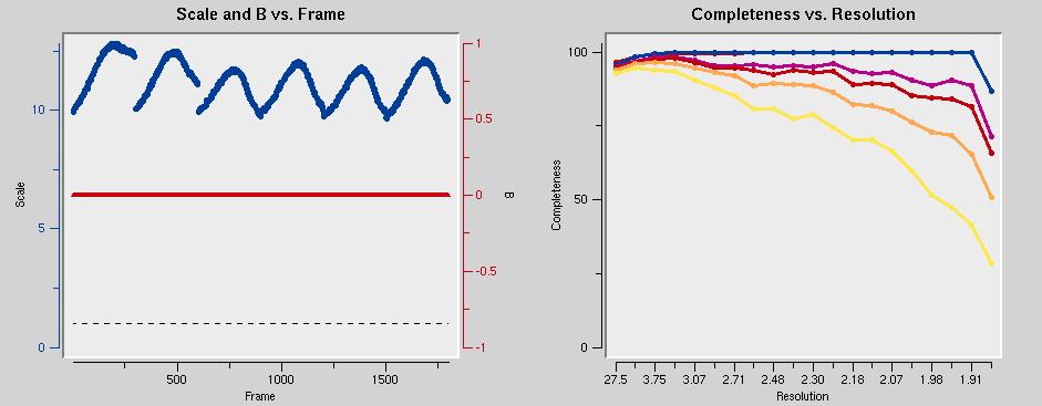
in addition, a number of graphs are generated that are worth inspecting. The scale factors (below left) should describe smooth curves. Outliers and discontinuities (except when going from dataset to dataset) are bad. You might want to exclude the offending frames by clicking on Exclude Frames. The graph below right shows that the data should be cut around 1.9 Å.
 The graph below left shows that the mosaicity is constant throughout all datasets. That's good. The graph on the right shows that the data are incomplete below about 25 Å. This is because of the beam stop shadow.
 The chi-square values below left should be around one. In the figure, they are too low. The error model needs to be adjusted to correct that.

From the initial scaling run, you can fill in the resolution cutoff values. Also, select Use rejections on next run to make sure that the reflections marked for rejection during the previous scaling are not used in the current run.

To adjust the error model, click on Adjust Error Model. A window will pop up as shown on the right. The errors should correspond to the linear R factor shown in the scaling statistics. It is unnecessary to modify them for each resolution shell. Instead, enter the overall value and hit Reset and Done.
In addition, decrease the Error Scale Factor in the main scaling window. This will increase chi values.
Scaling is an iterative process. It's done when the error model can't be improved further. Until this is done, keep cycling from adjusting scaling parameters to scaling to inspecting the results.
If you feel you're not quite getting there, you can select Use Auto Corrections in the main window.
In the end, the chi-squared graph should look like the one shown below. Also note how in the R-factor vs. Resolution graph shows higher R factors for unmerged intensities (green curve) than for merged intensities (blue curve). This is evidence of anomalous signal. Obtaining phases is straightforward from these data.
 The output file (output.sca) can be used directly in Shelx or converted to mtz with ccp4 tools.

