Magnetometer

References are in bold and can be found in the references section below. Figures and tables are also highlighed in bold and can be viewed below.

The simple, spherically symmetric and time-independent model of hydrodynamic expansion of the solar corona proposed originally by Parker (1963) has provided a useful framework for describing interplanetary observations of the solar wind and of the interplanetary magnetic field (e.g. Balogh 1985). However, observations of the Sun and of the solar corona, as well as direct and indirect interplanetary measurements clearly indicate that there are very significant departures from both spherical symmetry and time independence (Hoeksema 1985). A range of temporal and spatial features have been observed and identified in the interplanetary medium, primarily originating in non-uniformities on the Sun and its atmosphere, but partly also as a result of dynamic evolutionary processes in interplanetary space. In most cases, there are significant uncertainties concerning the heliolatitude dependence of interplanetary phenomena which have so far been observed only in and near the ecliptic plane. There is a need for direct observations to be made over a wide range of solar latitudes, hence the need for the Ulysses mission.

The heliospheric magnetic field, embedded in, and transported by the highly conductive solar wind, originates in the solar surface field. The interaction between the coronal plasma and the magnetic field generates the large diversity of structures in the solar atmosphere, with the dominant time scales probably determined (ultimately) by the evolution of the subsurface magnetic field. These time scales vary from minutes to the 11 year solar activity cycle, or even to the 22-year solar magnetic cycle. Time scales at the shorter end of the range affect the interplanetary medium mostly through the consequences of intense but transient phenomena such as solar flares and coronal mass ejections. However, large variations at the scale of a few minutes in the interplanetary magnetic field might originate, as in the case of Alfven waves, at or below the photosphere. Longer time scales are associated with relatively stable and large scale coronal structures. Most of the steady state solar wind is associated with coronal holes, with open magnetic field lines extending into interplanetary space (Hundhausen 1977).

While there is great variability in the strength of the magnetic field in interplanetary space, reflecting both coronal variability and the effects of solar rotation, it has been found that the long-term average field direction is closely following the Parker model (Thomas & Smith 1980). However, at large heliocentric distances, close to the ecliptic, there is evidence that the magnitude of the field decreases more rapidly than predicted by the Parker model (Winterhalter et al. 1990, see also Klein et al. 1987 for an alternative view), indicating that there may be large scale deviations from that simple model.

It has been suggested that the large scale structure of the heliospheric magnetic field over the solar poles may deviate significantly from the Parker spiral (Jokipii & Kota 1989). This would be due to residual transverse fields close to the sun decaying only as the inverse of the heliospheric radial distance, whereas the radial component decays proportionally with the square of the heliospheric distance. Therefore, even small deviations from the radial field close to the sun can lead to large deviations from the spiral field. The magnitude of this effect at the polar distances of Ulysses (between 2 and 3 AU) is somewhat speculative, but magnetic field measurements, together with energetic particle measurements (which "sample" the magnetic field structure over larger distance scales) will provide a test of this theoretical model.

The sector structure, which consists of the magnetic field vector pointing, on average, towards or away from the sun along the Parker spiral, as observed in and near the ecliptic plane, is the consequence of the heliospheric current sheet, separating field lines extending from the two solar hemispheres dominated by opposite magnetic polarities (Hoeksema et al. 1983). The global shape of the heliospheric current sheet has been successfully correlated with the neutral line at a solar wind surface obtained by extrapolating the photospheric magnetic field into the corona at 2.5 R ₀ (e.g. Smith et al. 1985). However, the extent to which solar wind dynamics influences the shape of the current sheet remains a topic of significant current interest.

The primar y scientific objectives of the magnetic field investigation on Ulysses, summarised in Figure 1 (see below), are formulated in terms of the expected evolution of already known structures and phenomena as a function of heliolatitude (Balogh et al. 1983). It is not known to what extent features in the corona will preserve their latitude dependence in the solar wind, and even their signature is difficult to predict. It is therefore possible only to indicate in qualitative terms the types of questions which will be answered by the Ulysses magnetic field observations. These can be classed as follows:

- questions concerning the large scale structure, in particular to what extent the Parker model is modified by the effects of the mid- latitude and polar field structures during the descending phase of the solar cycle; this heading also includes the latitude gradients in the field;
- questions concerning dynamical features arising from different velocity solar wind streams interacting in interplanetary space;
- questions concerning waves, discontinuities and transient phenomena, in particular the latitudinal extent and propagation of shocks.

The investigation also provides an opportunity to revisit some of the questions concerning the in-ecliptic magnetic field at this post-maximum phase of the solar cycle.

Finally, the Jupiter flyby needed for achieving the out of ecliptic orbit provides an opportunity to explore magnetic field features in the high latitude dusk regions of the Jovian magnetosphere.

In cooperation with other investigations, the magnetic field observations will also provide the framework for studies of energetic particle propagation in the high latitude heliosphere, in particular to address questions concerning the access and propagation of galactic cosmic rays.

References are in bold and can be found in the references section below. Figures and tables are also highlighed in bold and can be viewed below.

2.1. GENERAL.

The instrument (first described in detail by Balogh et al. 1983) consists of two magnetometers and of an on-board data processing unit. The two magnetometers have adequate sensitivity and sufficiently low intrinsic noise to measure the weak interplanetary magnetic fields at large heliocentric distances. The two tri-axial sensors use different physical principles to measure three orthogonal components of the magnetic field vector. This approach has not only the advantages associated with the dual magnetometer technique for detecting any background field due to the spacecraft, but also provides an independent means for evaluating the self-consistency of the measurements made by the two sensors.

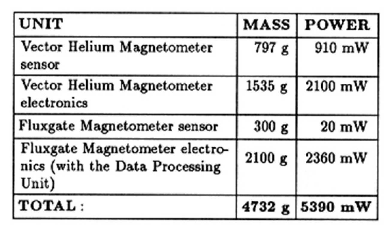
The overall block diagram of the flight instrument is shown in Figure 2. The Vector Helium Magnetometer (VHM), with its associated electronics unit, was designed and built by the Jet Propulsion Laboratory; the Imperial College team provided the Fluxgate Magnetometer (FGM) and its associated electronics, as well as the Data Processing Unit (DPU) for both magnetometers. The mass and power requirements of the instrument are given in Table 1 (right). The Experiment Ground Support Equipment used for spacecraft level tests of the instrument was also provided by Imperial College.

The two magnetometer sensors are located on the radial boom of the Ulysses spacecraft: the VHM sensor at the end of the 5 m boom, the FGM sensor at 1.2 m inboard from the VHM. Using magnetic mapping and modelling and appropriate compensation, the background field of the spacecraft at these locations was determined, prior to launch, to be approximately 30 pT and 50 pT, respectively; this makes the Ulysses spacecraft probably the magnetically cleanest interplanetary probe ever flown. The 3D magnetostatic profile of the spacecraft is shown in Figure 3 (kindly provided by Mehlem, 1989). This result has been achieved by a strictly enforced magnetic cleanliness programme, supported by extensive unit and system-level testing and modelling. The Flight Model spacecraft was tested twice in the large magnetic test facility of IABG, Ottobrunn, Germany, once in 1983, and again in 1989, when it was found that over that long interval there was effectively no significant change in the very high magnetic cleanliness level of the spacecraft. A few localised strong magnetic field sources in the spacecraft (the Travelling Wave Tubes and one of the experiment units) were locally compensated. The spacecraft power source, the Radioactive Thermoelectric Generator (RTG) was found to contain a stable but large intensity current loop; the magnetic field due to this source was also successfully compensated, using highly stable magnets, after an extensive test and modelling programme. In flight, the two magnetometers have been able to confirm the order of magnitudes of the pre-launch estimates of the spacecraft background field. (Due to unavoidable background disturbances, it is difficult to measure offsets on the ground with an accuracy better than about 0.1 nT. In orbit, however, offsets can be determined to a significantly greater accuracy).

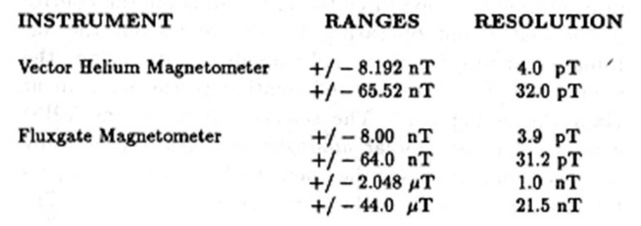
The prime scientific function of the instrument is to provide a time series of samples of the magnetic field vector along the trajectory of Ulysses. The overall performance characteristics of the instrument are summarised in Table 2 (left). The high speed digital data stream consists of vector samples at rates up to two vectors per second, depending on the data rate of the spacecraft telemetry. An auxiliarly low speed analogue data stream, despun onboard and digitised in the spacecraft housekeeping telemetry, originally foreseen to be distributed to other investigators for preliminary data analysis, does not appear to provide usable data. An event detector, responding either to large and sudden changes in the field component along the spacecraft spin axis or to large values of the rms of its variations, provides a flag for the speedy identification of potentially interesting events. Timing of this flag can be performed with high accuracy, through the spacecraft datation channel, in order to provide the timing of shock fronts or discontinuities with better precision than through the digital data channel.

2.2. THE VECTOR HELIUM MAGNETOMETER.

The VHM on Ulysses was developed from instruments flown successfully on the Pioneers 10 and 11 missions and on the International Sun-Earth Explorer 3/International Cometary Explorer probe (Frandsen et al. 1978). The schematic diagram of the VHM sensor is shown in Figure 4.

The operating principle of the VHM is based on the effect an ambient magnetic field has on the efficiency with which a metastable population of He gas in the triplet ground state can be optically pumped (Smith et al. 1975). In optical pumping, an incident radiation produces a distribution of atoms in non- thermodynamic equilibrium among the various energetic substates. In the VHM, circularly polarised light of wav elength 1.08 µm, generated in the lamp, is passed through the He cell, inducing an optically pumped metastable He population. The presence of an ambient magnetic field affects the pumping efficiency; the silicon infrared detector detects the consequent changes in absorption in the He cell, thus providing, for a constant lamp output, the change in the pumping efficiency. This depends not only on the magnitude of the magnetic field, but also on its angle with respect to the optical axis of the system.

Rotating magnetic fields are generated in the cell, alternately in two orthogonal planes intersecting along the optical axis of the sensor, using a three-axis Helmholtz coil system. The pumping efficiency, and therefore the detector output, vary as the vector sum of the sweep field and the component of the ambient field in the sweep plane. Phase coherent detection in the electronics produces output voltage signals representing the components of the ambient field along the optical and transverse axes alternately in the two orthogonal planes. These voltages are used to generate feedback currents in the Helmholtz coils so as to null the ambient field. The feedback currents provide highly linear measures of the three orthogonal components of the magnetic field vector in a reference frame defined with respect to the geometry of the sensor.

The VHM electronics unit generates the RF power used to produce and sustain discharges in the lamp and the cell, provides the sweep drive to the Helmholtz coils, processes the sensor output, generates an in-flight calibration reference, executes the commands for the control of the instrument operating modes, carries out the automatic ranging function and provides at its output the science and housekeeping information to the instrument Data Processing Unit. The science output of the VHM consists of three bipolar analogue voltages, representing the three components of the magnetic field vector, low pass filtered using a 0 to 4 Hz third order Bessel filter. The field equivalent noise of the VHM is about 3 pT/Hz^1/2.

The VHM has two operating ranges. Range 0 corresponds to a full scale of +/-8.190 nT, equivalent to a sensitivity of 1.60 nT/V; the full scale of range 1 is +/-65.52 nT, equivalent to 12.8 nT/V. In the automatic ranging mode, the instrument switches from range 0 to range 1 immediately if the voltage corresponding to any of the three components exceeds a preset threshold; it switches from range 1 to range 0 if all three components remain below a threshold value (approximately 10% of range 1 full scale) for a period longer than a full spin of the spacecraft. Automatic ranging can be overridden by ground command.

The VHM sensor has an electrical heater element, controlled from the electronics unit, to ensure a stable temperature for the sensor over the mission.

2.3. THE FLUXGATE MAGNETOMETER.

The triaxial Fluxgate Magnetometer (FGM) is an improved version of other instruments flown previously by the Imperial College, London team (Hedgecock 1975a). It is essentially similar to the fluxgate magnetometers flown by several other investigators on a variety of space missions. The FGM sensor consists of three identical single axis ring-core fluxgate sensors, arranged in an orthogonal triad, as shown in Figure 5. The operational block diagram of one of the axes is shown in Figure 6. Each sensor element consists of a high permeability ring core, with a toroidal primary winding, a rectangular secondary winding with its axis in the plane of the sensor core, and a calibration winding. The primary windings are driven by a 3675 Hz exponentially shaped bi-directional current pulse train, optimised to minimise the sensor noise. In the presence of an external magnetic field, a second harmonic of the drive signal ( 7350 Hz) is generated in the secondary winding, with an amplitude which is proportional to the component of the external field along the axis of the secondary winding. The phase of the signal with respect to the primary drive represents the direction of the magnetic field component. The signal from the secondary winding is amplified and band-pass filtered, then fed to a phase sensitive detector whose output is integrated. The output of the integrator is fed back to the secondary winding through one of three feedback paths to null the input signal. The feedback signals to the three sensors represent in magnitude and sign the three components of the ambient magnetic field vector from the sensor. A further switchable x 8 amplifier and a third order Bessel filter complete the processing chain for each sensor.

The switchable feedback paths and output amplifier provide the four ranges for the FGM. These are +/-8 nT, +/-64 nT, +/-2048 nT, and for pre-launch tests in the Earth's field, +/-44000 nT. Range switching for the FGM is by ground command only. The calibration coils wound on the three sensors are used for one of the FGM in-flight calibration modes.

2.4. THE ONBOARD DATA PROCESSING UNIT.

The functions of the Data Processing Unit comprise the execution of telecommands to control the operating mode of the whole instrument; the collection and onward transmission of digital status and analogue housekeeping data; analogue despinning and low pass filtering of data from the magnetometers; event detection; digitisation and formatting of magnetometer data for transmission to the spacecraft telemetry system.

The instrument status is set by dedicated telecommands from the ground. Two operationally identical 16bit command words, which can be used redundantly, control the operating modes of the VHM and FGM magnetometers, as well as those of the DPU. Commands which merit special mention are the safing of the VHM in high fields (during the Jupiter flyby, when the instrument remains switched on, but the ignition pulses to relight the lamp - already lit - are inhibited during the eventual saturation near closest approach); manual override range commands for the VHM; range commands for the FGM; calibration commands to both VHM and FGM, including the initiation of the special automatic in-flight calibration sequence which is described further below; selecting between two event selection criteria and, independently, between a low and high trigger threshold for the event detector. The receipt of commands is acknowledged through the digital status information transmitted through the telemetry.

Commands also define the modes of digital data acquisition. The switching pattern of the data flow through the DPU is shown schematically in Figure 7. The instrument has two parallel data acquisition and formatting channels, matching the two independent digital science data channels to the spacecraft. Each channel contains a 12-bit analogue-to-digital converter, the associated timing and control logic, and an output buffer register to the spacecraft. The two magnetometers can be connected to either or both these channels. Sampling is carried out at a uniform rate, to ensure that for any combination of sensors selected at the input, a uniform time series of vector measurements is generated by the instrument.

Vector samples are generated in synchronism with the data transmission rate. At the highest telemetry rate (1024 bps), two ve ctors are transmitted per second, and proportionally lower rates at lower telemetry rates. Digital science data are transmitted in blocks of 5 bytes, or 40 bits. Each vector measurement consists of 3 x 12 bits representing the X-, Y-, and Z components of the magnetic field vector, resp ectively. Three flag bits are transmitted to indicate the source of the data (VHM or FGM), as well as the range of the instrument being sampled. Finally, as a data quality check, a single parity bit is transmitted, generated from the whole vector block. Vector samples are transmitted alternately through the two digital science channels, so that in the case of the two magnetometers being connected through the two parallel data channels (as in the current early orbit operations), they generate an interleaved set of samples, uniquely recovered from the two science channels during the data processing stage.

The three components of the magnetic field vector are measured in a coordinate system fixed with respect to the geometry of the sensors which is also fixed with respect to the mechanical axes of the spacecraft. One axis of each magnetometer sensor is aligned with the spin axis, while their other two axes are in the plane perpendicular to it. For a constant (near DC) magnetic field, the sensors measure two rotating field components in the spin plane.

Onboard analogue processing of the data includes the generation of a low-pass filtered (0.01 Hz) vector set, in analogue form, transmitted through the spacecraft analogue housekeeping channels. These data are despun onboard, using an approximate despinning algorithm, based on Walsh transforms, driven by the spacecraft-provided sun pulse and spin segment clock. The vectors are rectified, to match the single-ended analogue interface, with the corresponding sign bits transmitted through the digital housekeeping channels. An estimat e of the spectral properties of the spin-aligned component of the magnetic field is obtained through a fourth analogue data channel, which is high pass filtered, rectified and time averaged through a 0.01 Hz filter. The frequency response of this channel, when used with the FGM, covers 4 octaves from 0.15 Hz to 1.2 Hz. All four channels are digitised by the 8-bit spacecraft analogue to digital converter.

2.5. IN-FLIGHT CALIBRATION.

Both magnetometers have in-flight calibration facilities to check periodically their scale factors during the mission. Two kinds of in- flight calibration modes are used. The first consists in superimposing on the measured field a calibrated step (or bipolar step, in the case of the VHM) for a fixed interval on all three axes. The second mode consists in superimposing a train of 512 on-off calibration steps, in synchronism with the vector sampling sequence, at half the Nyquist frequency. The analysis of the calibration data can be carried out in the frequency domain, and the step size can be recovered in the presence of variable fields (which, on the two axes perpendicular to the spin axis, vary sinusoidally even in the presence of a constant ambient field). Calibration data show that the step height can be recovered with an accuracy better than 1 part in 1000.

2.6. IN-ORBIT PERFORMANCE OF THE INSTRUMENT.

The instrument was switched on in orbit on 25 October 1990. Following a full in orbit checkout, it was noted that the data from the two onboard despun analogue channels were unusable. As both channels are affected, the signal chain from the spacecraft sun pulse and spin segment clock is the assumed cause of the observed symptoms. As these data were to be automatically distributed to other investigators for preliminary data processing purposes, alternative arrangements were immediately made to generate a data set of similar time resolution (four minute averages), but of much higher quality, from the processed digital science data. The task of providing high quality averaged data for inclusion into the widely distributed Common Data File has been undertaken by the JPL members of the magnetometer team.

The prime science data from the instrument has proved to be of the expected high quality. Following initial compatibility tests between the VHM and FGM sensors, the instrument was left operating using both sensors, with the VHM in auto-ranging mode, and the FGM in its +/-64 nT range. The VHM sensor heater was switched on to provide a stable temperature for the sensor. The FGM sensor, not having been provided with a heater, is following the expected large drop in temperature as the spacecraft moves further away from the sun. As a result, the offset of the Z component of the FGM has drifted, but as any drifts (well within range) can be derived (see below), full correction is routinely made during the preliminary stages of the data processing. All three axes of the VHM show very small and stable offsets, as do the two other axes of the FGM as well. Preliminary sensitivity (scale factor) comparisons between the two sensors show a very good match. Overall, with all currently implemented corrections carried out, the two sensors are inter-calibrated to better than 0.1 nT. Use of the two different sensors simultaneously provides a very high confidence in the quality of the data.

2.7. GROUND DATA PROCESSING.

The data processing flow for the magnetic field investigation, from raw data to the standard data sets for scientific analysis, is shown in Figure 8.

The primary means of magnetic field data being made available to the magnetometer experiment team is by the EDR (Experiment Data Records) tapes. This contains the subset of the raw telemetry data relevant to the magnetometer. The first stage of pre-processing of the EDRs is to extract the digitised field components from the data stream along with instrument status words and engineering data. A number of quality and consistency checks are made on the data so that any bad vectors are not processed further. The engineering data is passed to a history file from where it can be later plotted. The instrument status words provide the operating range(s) of the instrument(s) on the two channels, thus allowing the appropriate calibration factors to be applied to convert the digitised field values into nT units.

If any in-flight calibration data is included in the data stream it is at this point fed out to a calibration file for later analysis. The remaining data is spin-averaged to provide a measure of the offsets affecting the X and Y (spin plane) sensors of the magnetometers. Time tagged values of the calibration constants and offsets are stored in a file. This file is accessed during a second pass through the data with the pre-processing software to allow corrections for any changes in calibration or offsets to be made. The data are then despun, i.e. transformed from the coordinate system with X and Y axes rotating with the spacecraft to one with the X and Y axes having a fixed direction in space.

Estimates of the offset on the Z axis sensor can now be made. This is done using the equivalent methods of Davis and Smith (1968) and Hedgecock (1975b) which work by finding the Z offset value which minimizes the covariance between fluctuations of the field magnitude and fluctuations in the angle that the field vector makes with the Z axis.

Finally, Reduced Data Records (RDR) are produced. The RDR file is intended to be the fundamental stored data set for the Ulysses magnetometer. Data in this file are fully quality checked, calibrated and offset corrected.

Attitude and position data for the spacecraft are provided on the SEDR (Supplementary Experiment Data Records) tapes. These are pre- processed to provide an online file of the parameters necessary to perform coordinate transformation on the field vectors. The default coordinate system used is the RTN system which is spacecraft centered, with the R axis radially outwards from the solar direction, the N axis northwards in the plane of R and the solar rotation axis and the T axis completing a right handed system. The full time resolution data are made available for science analysis by passing it through a coordinate transformation software package which operates on the RDR file. Averaged data sets are made available by first averaging and then performing the coordinate transformation. It is intended to maintain a 1 vector per spin stored data set in RTN coordinates as well as to produce 1 vector per minute summary plots to identify periods of interest. One longer term averaged data set and summary plots will also be produced.

The RDR files are also used in the generation of 256 second averages for inclusion in the CDF (Common Data File).

As well as the EDR tapes, some data are also obtained routinely from the QEDR files (Quick Look EDR) available by Decnet remote access to the Data Records System at JPL within a few hours of being received from the spacecraft. The pre-processing of these is basically the same as applied to the EDRs except that temporary calibration and offset parameters are produced and used for generating quick look plots of the magnetic field. The QEDR allows a daily check to be made on the health and performance of the magnetometers and enables the team to make early decisions on whether instrument mode change commands are necessary. The QEDR facility has proved extremely useful and will be the primary means of accessing magnetic field data during Jupiter encounter.

References are in bold and can be found in the references section below. Figures and tables are also highlighed in bold and can be viewed below.

3.1. GENERAL.

The first data analysis task has been the validation of instrument performance in flight. As already stated, the early in orbit data showed the two magnetometer sensors to be intercalibrated to better than about 0.1 nT, thus confirming the pre-flight tests carried out in the IABG magnetic facility.

During the period November and December 1990, the spacecraft was nutating, due to the differential heating of the axial boom of the wave experiment. Members of the magnetometer team at JPL (Smith & Wigglesworth) used the magnetometer data to provide supporting analysis for the spacecraft flight dynamics team, exploiting the sensitivity of the frequency domain analysis techniques to measure the nutation angle. A sample power spectrum is shown in Figure 9, exhibiting two narrow peaks at [OMEGA]₀- [omega] and [OMEGA]₀ + [omega], where [OMEGA]₀ is the spin frequency and [omega] is the nutation frequency. The power at these frequencies can be converted to the equivalent signal amplitude and then into the maximum nutation angle. At this time, the half cone angle the nutation was 1.5°. Note that the nutation peaks are superimposed on the typical interplanetary power spectrum following a f ^-3/2 dependence. The observations from late October 1990 to March 1991 show that the interplanetary field at this phase of the solar cycle is highly disturbed: several potential shock waves and a large number of rotational and tangential discontinuities have been observed. At this stage, only data from the magnetometers has been analysed; in many cases, more fruitful analysis awaits the start of routine data exchanges with other investigators on Ulysses. In the following, we present a sample of observed phenomena over the first few months of observations.

3.2. WAVE BURSTS ON 29 OCTOBER 1990.

Only four days after the switch-on of the instrument, a period of intense wave bursts was observed by the magnetometer. At first, only a period of some 20 minutes was identified, as shown in Figure 10. However, closer inspection of the data later on the same day showed that the wave activity persisted up to 14 hours later, if less noticeably, as during the later periods the fluctuations were only seen in the components and not in the magnitude of the magnetic field. (Artificial causes of the wave activity, due to instrumental or spacecraft effects were eliminated early on in the analysis). Power spectra of the spin-aligned component of the magnetic field are shown in Figures 11a and 11b, showing large and broad peaks, with the maximum at 0.2 Hz and 0.1 Hz, respectively for the earlier and later periods. The peak power was about 2 (nT)²/Hz for the period from 05:04 to 05:23 UT, and 3 (nT)²/Hz from 19:20 to 19:39 UT. A principal axis analysis has s hown that the waves during the earlier period were elliptically polarised, mostly in a left-handed sense, but with up to 20% of the time in the right handed sense in the spacecraft frame. The origin of this very unusual event has not yet been established.

3.3. CROSSING OF THE HELIOSPHERIC CURRENT SHEET ON 9 NOVEMBER 1990.

The spacecraft crossed the heliospheric current sheet twice on that day, first at about 10:25 UT, then again about 19:26 UT, as shown by the reversals in the field direction in Figures 13a and 13b. The first reversal was slower than average, lasting about four minutes, and with significant noise at the current sheet. A principal axis analysis of the first crossing has shown that the field rotated through less than 180°, with very nearly constant magnitude; the analysis has also indicated that there may have been a significant non-zero normal field component. The second crossing, still with nearly constant magnitude, was more rapid (less than 1 minute). Several such crossings were observed and will be analysed in detail later.

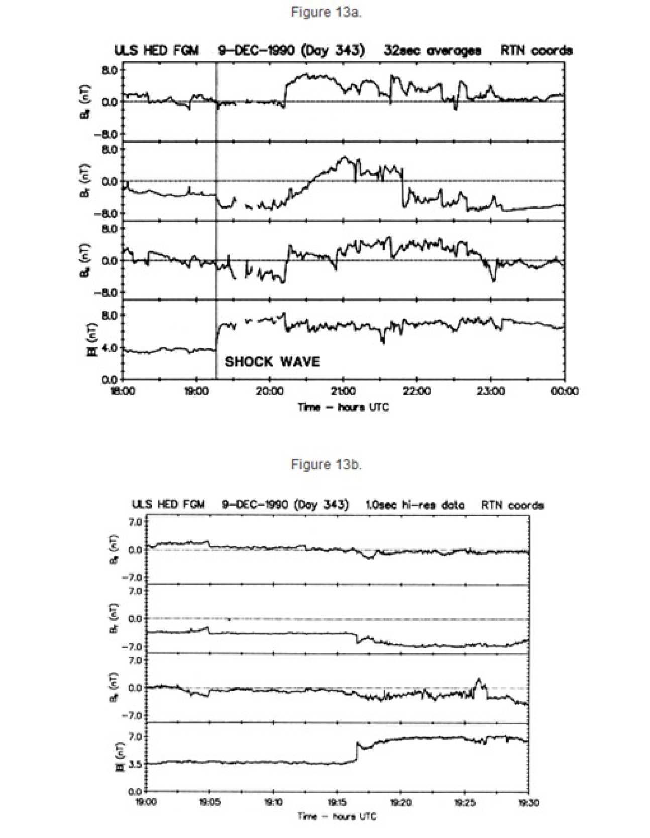
3.4. INTERPLANETARY SHOCKS ON 9 DECEMBER 1990 AND 31 JANUARY 1991.

The magnetometer has observed several candidate shock events during the first months. Most of these remain to be confirmed, but there is little doubt concerning several of these events. Two examples are given. The first, on 9 December 1990 at 19:17 UT, shown in Figures 12a and 12b appears to be a fast forward shock, very likely to be the same shock that was observed by IMP 8 on 8 December. (This was also the time of the Galileo Earth flyby). The second example is a reverse shock observed on 31 January 1991 at 04:12:30 UT. A principal axis analysis was carried out on this event, not usually appropriate to shocks because the change is normally uni- directional. However, the analysis indicates that there appears to be a significant out-of-plane component, i.e. a component perpendicular to the "co-planarity" plane. This is a rare observation for interplanetary shocks, although common to observations of the Earth's bow shock. Further analysis is being carried out on this, as on other shock events.

The successful implementation of the Magnetic Field Investigation has been the result of much dedicated effort by many people over many years. At Imperial College, Mrs Anne Hedgecock laid the foundations for the data processing software. At the Jet Propulsion Laboratory, important contributions to the instrument were made by A.M.A. Frandsen, B.V. Connor, J. van Amersfoort, E.W. Noller, R.N. Miyake and J. Cravens. The successful implementation of the data processing effort at JPL has been carried out by L. Wigglesworth and J. Wolfe.

We thank members of the Ulysses Project Teams, led with determination by the Project Managers, Derek Eaton and Willis Meeks, and their spacecraft and payload support teams. Very many individuals in the ESA and JPL Project Teams contributed to the success of the mission over the years: Peter Casely, the late Mike Agabra and Tom Tomey in particular provided much direct help to experiment. Significant support, gratefully acknowledged, was also received from Dieter Kolbe and his colleagues in the Dornier team. We would also like to thank the F ESOC Operations Team (in particular Peter Beech and Nigel Angold) for their helpfulness, and the JPL Data Management Team for their efforts to provide us with usable data to date and in the future.

Special thanks go to the ESA Project Scientist, Dr. K.P. Wenzel and his Deputy, Dr. R. Marsden, for the support they have given to our team and for their many vital contributions to the mission as a whole. The magnetometer team as a whole wishes also to thank one of the co-authors of this paper, Dr. E.J. Smith, who in his capacity as NASA Project Scientist has greatly contributed to the success of Ulysses.

Ulysses has set new standards in magnetic cleanliness, thanks to the sustained efforts of the ESA, JPL and Dornier Project Teams. The modelling and analysis work was carried out by Dr. K. Mehlem of ESA.

The Imperial College contribution to the Ulysses magnetic field investigation has been supported by the U.K. Science and Engineering Research Council. Some of the research described in this publication was carried out by the Jet Propulsion Laboratory, California Institute of Technology, under a contract with the National Aeronautics and Space Administration.

Balogh A. 1985, in The Sun and the Heliosphere in Three Dimensions, R.G. Marsden Ed.

(D. Reidel Publ. Co.) p. 255

Balogh A., Hedgecock P.C., Smith E.J. and Tsurutani B.T. 1983, in The International

Solar Polar Mission Its Scientific Investigations, K.P. Wenzel, R.G. Marsden and B.

Battrick Eds, ESA SP-1050, 27

Davis L. Jr. and Smith E.J. 1968, Trans. AGU 49, 257

Frandsen A.M.A., Connor B.V., van Ammersfoort J. and Smith E.J. 1978, IEEE Trans.

Geosci. Electron. GE16, 195

Hedgecock P.C. 1975a, Space Sci. Instrum. 1, 61

Hedgecock P.C. 1975b, Space Sci. Instrum. 1, 83

Hoeksema J.T. 1985, in The Sun and the Heliosphere in Three Dimensions, R.G.

Marsden Ed. (D. Reidel Publ. Co.) p. 241 Hoeksema J.T., Wilcox J.M. and

Scherrer P.H. 1983, J. Geophys. Res. 88, 9910

Hundhausen A.J. 1977, in Coronal Holes and High Speed Solar Wind Streams, J.B. Zirker

Ed. (Boulder: Colorado Associated University Press) p. 225

Mehlem K. 1989, ESTEC Working Paper EWP-1564, Noordwijk

Jokipii J.R. and Kota J. 1989, Geophys. Res. Let. 16, 1

Klein L.W., Burlaga L.F., Ness N.F. 1987, J. Geophys. Res. 92, 9885

Parker E.N. 1963, Interplanetary Dynamical Processes, Interscience Publishers

Smith E.J., Connor B.C. and Foster G.T. Jr. 1975, IEEE Trans. Magn. MAG-11, 962

Smith E.J., Slavin J.A. and Thomas B.T. 1985, in The Sun and the Heliosphere in

Three Dimensions, R.G. Marsden Ed. (D. Reidel Publ. Co.) p. 267

Thomas B.T. and Smith E.J. 1980, J. Geophys. Res. 85, 6861

Winterhalter D., Smith E.J., Wolfe J.H. and Slavin J.A. 1990, J. Geophys. Res. 95, 1

Figure 1. A schematic summary of the scientific objectives of the magnetic field investigation on Ulysses. The questions to be answered by this mission are formulated in terms of the heliolatitude dependence of phenomena and structures observed close to the ecliptic plane.

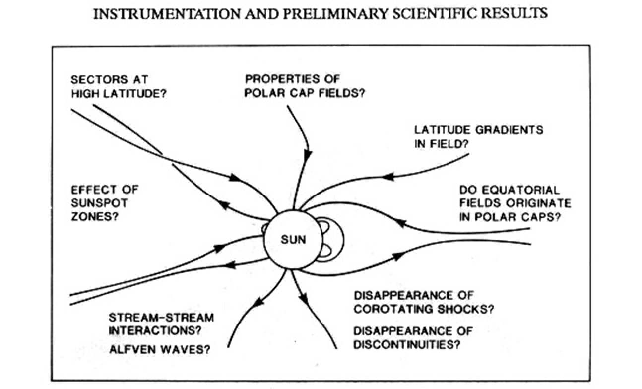
Figure 2. The block diagram of the flight instrument on Ulysses for the measurement of the magnetic field vector along the orbit of the mission. The two magnetometer sensors are located on a 5 meter boom, while the electronics unit (comprising the units designated as HED1 and HED2) are located within the spacecraft. The HED1 and HED3 units have been provided by Imperial C ollege London, and the HED2 and HED4 units by the Jet Propulsion Laboratory.

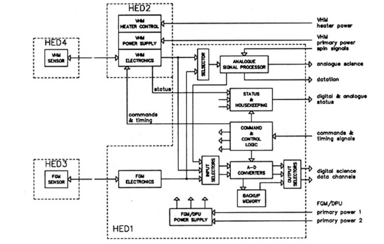
Figure 3. A contour plot representing the magnetic field model of the Ulysses spacecraft (Mehlem 1989), based on extensive measurements carried out on the flight spacecraft in the Magnetic Test Facility of IABG (Ottobrunn, Germany) Both magnetic mapping and modelling indicate the unparalled cleanliness of the spacecraft, confirmed in flight.

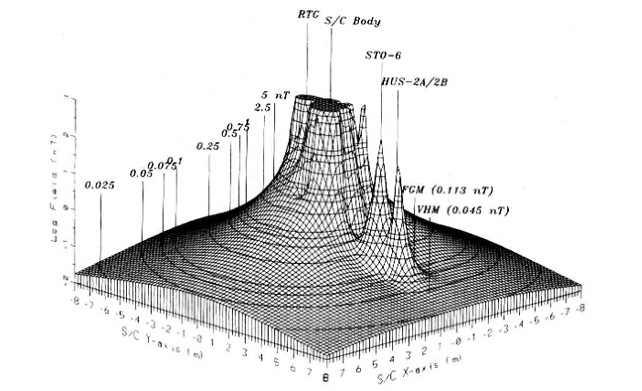
Figure 4. A schematic diagram of the Vector Helium Magnetometer sensor. The optical axis of the sensor is aligned with the spacecraft boom. For the sake of clarity, the third set of Helmholtz coils, completing the orthogonal triad, have been omitted from the drawing.

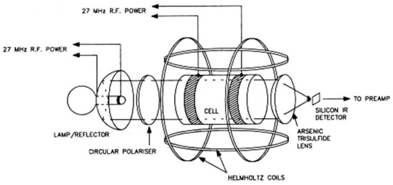
Figure 5. A schematic diagram of the three orthogonally arranged uni-axial ring-core sensors in the tri- axial Fluxgate Magnetometer sensor, placed on the spacecraft boom. The alignment of the sensors was determined prior to launch to better than 0.1°.

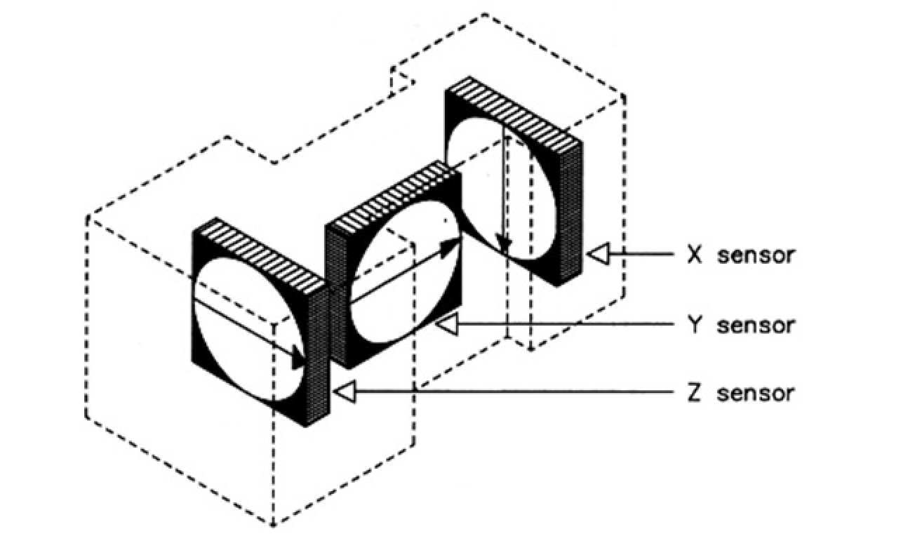
Figure 6. Schematic diagram of the electronics signal chain for one of the three axes of the Fluxgate Magnetometer. The drive electronics is common to all three axes up to the complementary symmetry switches. Different ranges are activated by switching the feedback circuits.

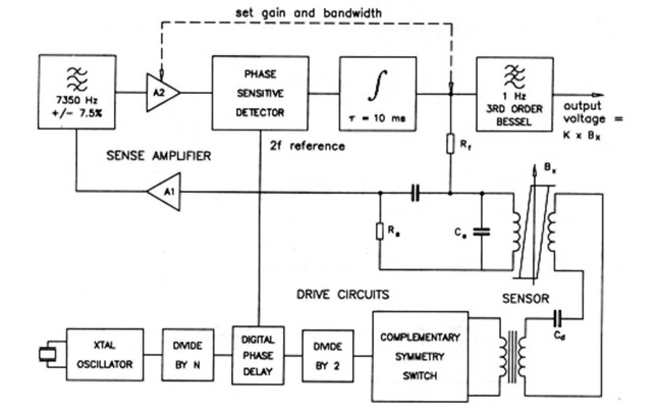
Figure 7. Block diagram of the digital onboard Data Processing Unit (DPU), serving both Vector Helium and Fluxgate Magnetometers. The schematic representation of switches activated by ground command shows the extensive redundancy built into the DPU.

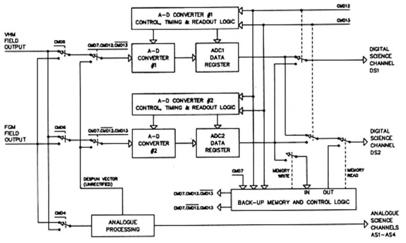
Figure 8. Flow diagram of the ground processing of the magnetic field data, from receipt of decommutated raw data from the Ulysses Data Managegment System at the Jet Propulsion Laboratory, to processed data products ready for scientific analysis by both the magnetometer team and for cooperative data analysis with other Ulysses investigators.

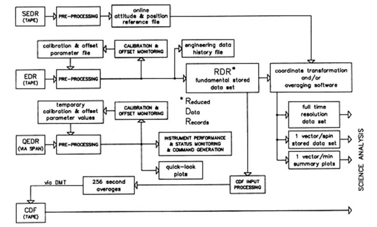
Figure 9. The power spectrum of the spin-axis aligned component of the magnetic field measured during the period in November 1990, when the spacecraft was nutating. The figure shows the superposition of two peaks at frequencies resulting from the combination of the spin and nutation frequencies on the background interplanetary field power spectrum. Detailed analysis indicates that these peaks corresponded to a nutation amplitude of 1.5°.

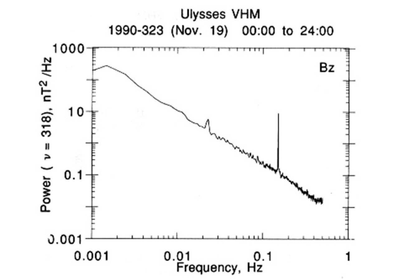
Figure 10. A highly unusual wave burst detected by the Ulysses magnetometer on 29 October 1990. Detailed investigations eliminated the possibility that the disturbances were caused artificially, although the natural cause remains to be firmly identified. This event (also illustrated on Figs. 11a and 11b below) is the subject of further investigation by the magnetometer team, made difficult by the fact that many other relevant instruments on Ulysses were not yet switched on at that time.

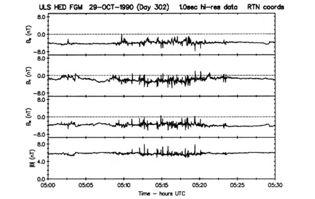
Figure 11a and 11b. Power spectrum (a) of the spin-aligned component of the magnetic field during the wave burst shown in Figure 10 (above), and power spectrum of the same component of the field some 14 hours later on the same day, indicating that there were also waves at a somewhat lower frequency (0.1 Hz vs. 0.2 Hz) at the later time, but with increased amplitude, although mostly in the components (therefore direction) rather than in the magnitude of the magnetic field.

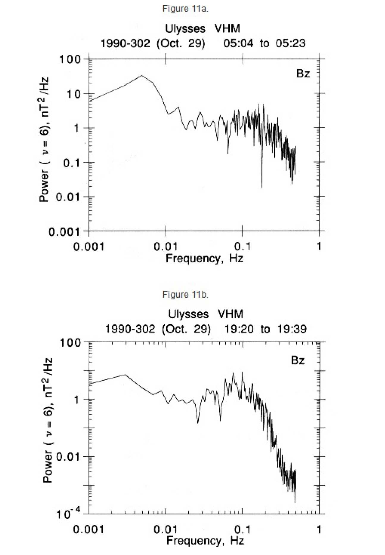
Figure 12a and 12b. Two crossings of the Heliospheric Current Sheet observed by the Ulysses magnetometer on 9 November 1990. The first crossing is relatively slow, with significant wave activity attached to it, while the second crossing is more typical of those seen by previous investigations.

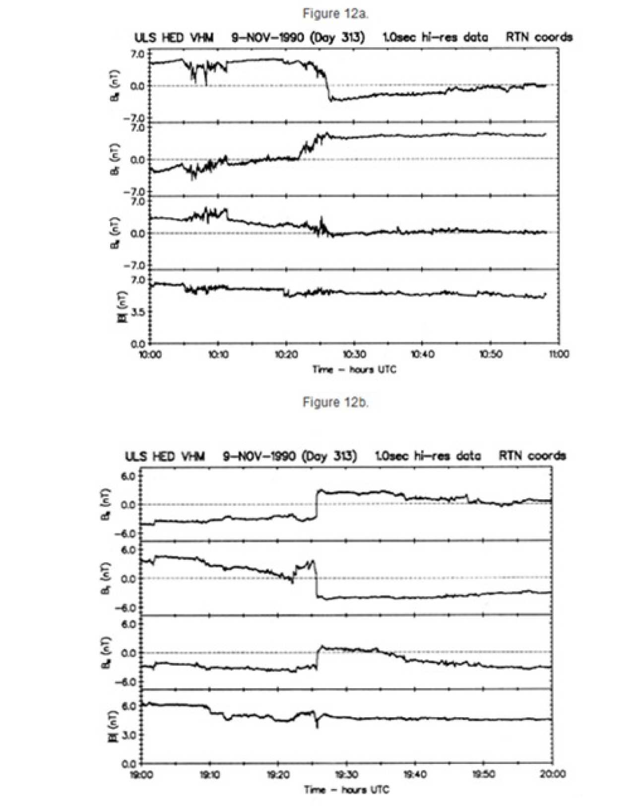
Figure 13a and 13b. One of the several shock waves observed by the Ulysses magnetometer to date. This is likely to be the same shock wave which was observed on the previous day by IMP-8 near the Earth (incidentally, during the Earth flyby by the Galileo spacecraft). Figure 13b shows at high time resolution the sudden increase of the field magnitude, likely to represent a near perpendicular fast shock. The large angular discontinuity observed about 1 hour after the shock passage was also apparently observed by IMP-8.