The behaviour of fluid flow is described by well-established partial differential equations – the Navier-Stokes equations - which are, essentially, particular forms of Newton’s laws of motion, supplemented by an equation describing the conservation of mass. Except for very simple conditions, these equations need to be solved numerically with the aid of computers (often super-computers). To this end, the predefined flow domain is covered by a numerical mesh, which defines nodes at mesh cross-sections and finite volumes or finite elements which are patches of area of volume cells around nodes or between consecutive mesh lines.

The differential flow-governing equations are then approximated, using numerical discretisation schemes, as sets of algebraic equations, each pertaining to a node, finite volume or finite element. The collection of coupled algebraic equation are then solved, by linear-algebra methods, on a computer to yield discrete values of velocity and pressure at mesh nodes. Additional transport equations may be solved, alongside the equations of motion and mass conservation, to calculate the temperature, species concentration, chemical reaction and multi-phase interactions (solid particles, bubbles, liquid droplets, etc.).

The collection of theoretical, numerical and computational techniques that facilitate this process is called Computational Fluid Dynamics.

Within the area of Computational Fluid Dynamics, some of the most challenging flows are those in which turbulence plays an important role – or, indeed, in which turbulence is the phenomenon of interest. Particular interest in turbulence derives from the fact that it is largely responsible for mixing, dispersion, frictional losses, vibrations and noise.

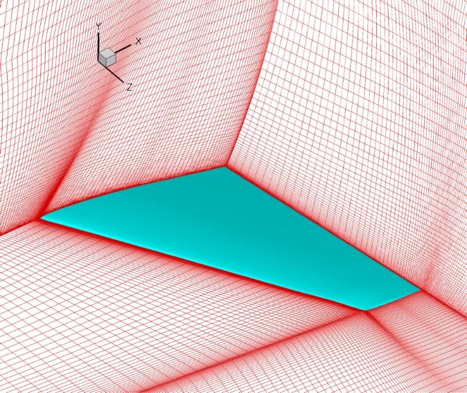
Being a highly effective mechanism for redistributing (mixing) momentum, turbulence has a major impact on gross aero- or hydrodynamic characteristics. It dictates, in particular, whether a near-wall flow remains attached or separated when subjected to adverse pressure gradient.

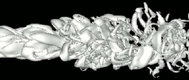
Any turbulent flow may be likened to contorted stream of fluid containing numerous mutually interacting, continuously changing eddies and vortices that move with the stream. This is illustrated by the snapshots below of a jet and a mixing layer undergoing transition and evolution towards a fully turbulent state. The vortices cover a wide range of size and time scales and change continuously in time and space as they evolve, stretch, deform and break up. These eddies are responsible for the high levels of mixing, diffusion and dissipation observed in turbulence.

Current approaches to computing turbulent flows fall under the headings of either simulation or modelling - a distinction pursued in the sub-section Simulation vs. Modelling.