2D detection of surgical instruments from the wearable camera and laparoscopic video

2D Detection

The results presented here can also be found in our paper: https://arxiv.org/abs/2209.05056

1.  Data Preparation

Data Collection

The endoscope dataset consists of two videos of a surgeon performing the laparoscopic cholecystectomy procedures on a patient using a standardized porcine model. Cholecystectomy, also known as gallbladder removal, is a tiny pouch-like organ located in the top right corner of the human stomach. Its responsibility is to store bile, a fluid released by the liver that assists in the digestion of fatty foods. Because humans do not require a gallbladder, surgical procedures to remove it are widely prescribed if a patient is experiencing any challenges with it. The endoscope videos were recorded using a high-definition camera (1080p, 1,920 x 1,080 resolution and progressive scan) Karl Storz, 30 degree, 10mm laparoscope. It is connected to a Karl Storz Image 222010 20 SCB Image 1 Hub Camera Control Unit. Before beginning the required annotation process, the video data collected as part of the MAESTRO Jr. AI project at Imperial College London was anonymized. Our aim in this section is to describe the various procedures employed in the data collection process, which includes the surgical task and the surgical phases involved in the data collection process. We also discuss the data annotation tool used for annotating the dataset, the data annotation protocols, and the data processing steps involved in preprocessing the data in order to prepare it for training.

Surgical tasks

The various surgical tasks involved in the data collection process include

• Laparoscopic cholecystectomy using a standardised porcine model.
• Body torso laparoscopic box trainer with prepositioned trocars. Possibly a haptic box trainer.
• Basic laparoscopic stack and standard surgical equipment (hook diathermy, Maryland graspers, crocodile graspers, 10mm and 5mm trocars, 5/10mm Endoclip applicator, Bert bag/Endocatch, 30-degree camera).

Surgical Phases

This subsection provides a brief description of the various surgical phases involved in the data collection process.

Retraction of the gallbladder: The surgeon passes the instrument(s) to the assistant surgeon, who holds the flaps up, in order for the surgeon to have a better view of the regions of interest, which are the gallbladder, liver, and cystic duct.

Dissection of critical view of safety: The surgeon uses hook diathermy and a Maryland grasper to dissect the hepatocystic/calot’s triangle.

Clipping and division of the cystic duct: The surgeon uses endoclip and laparoscopic scissors to clip the region of interest, which in this case is the cystic duct.

Clipping and division of the cystic artery: The surgeon uses endoclips and laparoscopic scissors to clip the region of interest, which in this case is the cystic artery.

Dissection of the gallbladder from the liver bed or cystic plate: The surgeon uses a crocodile grasper and hook diathermy to dissect the gallbladder from the liver bed. This causes the presence of smoke in the surgical scene.  

Removal of the gallbladder: The surgeon uses a Bert bag or Endocatch to remove the gallbladder from the surgical scene.

It is worth mentioning at this point that the participants involved in the data collection process are high surgical trainees specialising in general surgery recruited from the Department of Surgery and Cancer, Imperial College London. The participants have previous exposure to basic laparoscopic surgical training as well as simulated and clinical exposure to laparoscopic surgical/cholecystectomy training.

2.  Data Annotation Protocol

For the object detection task, the endoscope videos were manually annotated by drawing bounding boxes around the tips of the surgical instruments of interest in each image frame and entering the corresponding class label associated with each bounding box. This is what we term the "ground truth labels." For this annotation task, we annotated eight different surgical instruments, which are: Crocodile grasper, Johan grasper, Hook diathermy, Maryland grasper, Clipper, Scissors, Bag holder, Trocar.

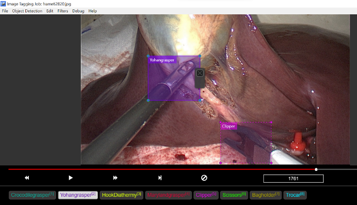
Figure 1: Screenshot of using Microsoft VoTT for annotating of our novel endoscope dataset.

3.  Data Annotation Tool

VoTT : The Virtual Object Tagging Tool (VoTT), which is a free and open-source data annotation tool from Microsoft, was used to annotate our endoscope video dataset. VoTT was used to draw bounding boxes around the tips of the surgical instruments of interest in our dataset. Figure 1 depicts a screenshot of its graphical user interface.

LABELME: LabelMe is a free open-source data annotation tool developed by MIT for manual image annotation for object detection, classification, and segmentation tasks. LabelMe was created in Python with the goal of collecting a large collection of images with ground truth labels. LabelMe is simple to use and lets you draw polygons, circles, rectangles, lines, line strips, and points, among other shapes. The Image below provides an overview of using LabelMe for image annotation.  A screenshot of the LabelMe annotation software is illustrated in Figure 2.

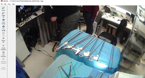
Figure 2: Screenshot of using Microsoft VoTT for annotating of our novel endoscope dataset. 

4.  Data Preprocessing

In order to make our novel endoscope data set ready for training, we performed a series of data preprocessing steps. We developed a python script to convert our novel endoscope videos into image frames. We implemented the Microsoft VoTT annotation tool for annotating the dataset and performed an adaptive image scaling operation to obtain a standard image size of 640×640 for training. The Microsoft VoTT annotation tool provides annotation of our dataset in MSCOCO data format, which is not the acceptable data format for YOLO algorithms. A python script was developed to convert the annotation from the MSCOCO data format to the YOLO data format.

5.  Methodology

YOLOv5 which is the fifth generation in the YOLO family, was released by Glenn Jocher and his research team at Ultralystics LLC a few months after the release of YOLOv4 by Bochkovskiy et al [1]. Earlier versions of the YOLO models were developed using a custom Darknet framework which is written in the C programming language. However, Glenn Jocher and his research team changed the trajectory by utilizing PyTorch, a deep learning library developed by the Facebook research team, which is written in the Python programming language, to build the YOLOv5 model. Small, Medium, Large, and Xlarge are the four distinct scales that YOLOv5 offers for their model. While the general structure of the model stays unchanged across the different scales, the size and complexity of each model is adjusted by a different multiplier for each scale. Although all our modifications and experiments were carried out using the large YOLOv5 model, it can still be replicated across other variants of the YOLOv5 model by adjusting the width and depth multiplier.

To establish a baseline, we trained and evaluated the unaltered YOLOv5 model on our novel endoscope dataset. Next, we implemented our proposed modifications (which we will discuss in the next session) on the YOLOv5 model, trained and evaluated its performance, and conducted an ablation study with our baseline unmodified YOLOv5 model. This procedure was repeated, monitoring if certain refinement strategies enhanced or compromised one another while gradually adding and removing more complex combinations. Finally, we benchmarked results from our unrefined and refined YOLOv5 models with results from YOLOv7, Scaled-YOLOv4, YOLOR, and YOLOv3-SPP models trained on our novel endoscope dataset. A comparison of their accuracy in detecting surgical instruments from endoscope videos and the identification of the best possible detector for our MAESTRO endoscope vision-based system. It is worth mentioning at this point that all models trained on our novel endoscope dataset were trained from scratch for 300 epochs without using pretrained weights.

Overview of Yolov5 Architecture

The YOLOv5 architecture, as illustrated in Figure 3, employs the Cross Stage Partial Darknet53 (CSPDarknet53) architecture and spatial pyramid pooling (SPP) layer as its backbone, the path aggregation network (PANet) architecture as the neck, and the YOLOv3 head for detection. The CSPDarknet53 module primarily extracts rich information from input images by performing feature extraction on the feature map. The output of the CSPDarknet53 is passed through the SPP layer before being sent to the neck for feature aggregation. The SPP layer, which is placed between the backbone and the neck, extracts important features from several scales into a single feature map, which increases detection performance. In the neck, the PANet architecture, which is an extension of the FPN with an additional bottom-up path, improves the ability of the model to detect objects at different scales by aggregating strong semantic feature maps from different feature layers. The head, which is the last step in the detection process, makes dense predictions on multi-scale feature maps from the neck module. The dense prediction consists of the bounding box coordinates (center, height, width), class label, and confidence score. To adapt to the differences in datasets, YOLOv5 incorporates the use of adaptive anchor box computation on its input. This allows the YOLOV5 model to automatically learn the best anchor box for any given dataset and utilise it throughout the training process [2].

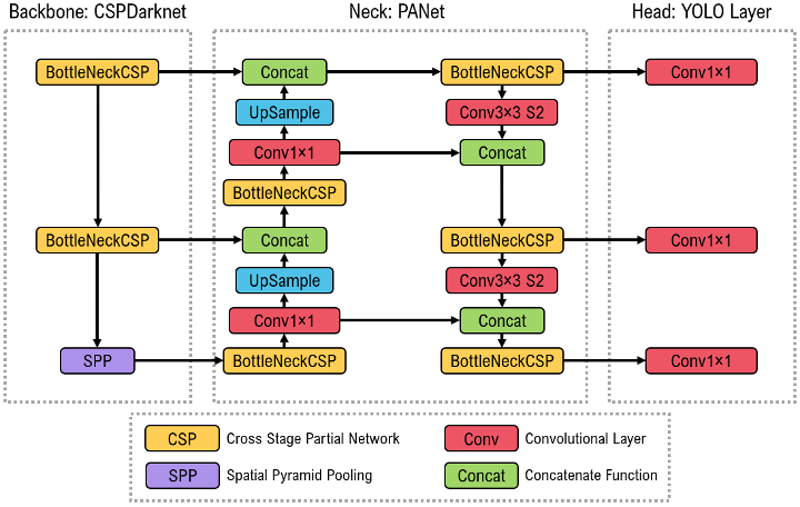
Figure 3: The unmodified YOLOv5 model's architecture, which is divided into three parts: Backbone:CSPDarknet with an SPP layer, Neck:PANet, and Head:YOLOLayer. The data is first supplied into CSPDarknet for feature extraction before being loaded into PANet for feature fusion. Finally, the YOLO Layer generates the object detection results (i.e., class label, class score, location, size) [3]

Our Modifications

The YOLOv5 model makes use of a .yaml file which contains instructions for the overall model architecture. These instructions are fed to the parser, which then builds the model based on the information in the .yaml file. In order for us to implement any modification, we emulated this arrangement by rewriting a new .yaml file containing our proposed modification to instruct the parser to build the model.

The key modifications that we proposed for the YOLOv5 models are in the backbone, the neck, and a few hyper-parameter changes in order to optimize model performance on our novel endoscope dataset. This modification was inspired because the original YOLOv5 model was trained on the MSCOCO dataset, which in all ramifications is a different dataset from our novel endoscope dataset. In this section, we will describe our proposed modification to the YOLO5 network in detail.

Backbone

The unmodified YOLOv5 model uses CSPDarknet as its backbone. In this work, we replaced the CSPDarknet backbone with a modified VGG-11 backbone by removing the fully connected layers in the original VGG-11 architecture and adding the SPP layer, which is an additional layer between the unmodified YOLOv5 backbone and neck. VGG, which stands for Virtual Geometry Group, was first proposed by A. Zisserman and K. Simonyan at the University of Oxford. They investigated the influence of convolutional neural network depth on accuracy in the context of large-scale image recognition [4]. Their main contribution was increasing the depth of the model by replacing large kernel-size filters with very small 3 x 3 convolution filters. This achieved significant improvement over prior art like AlexNet [5] and almost 92.7% top-5 test accuracy on the ImageNet dataset.

Neck

The neck in the YOLOv5 is the series of layers between the backbone and the head. The unmodified YOLOv5 model uses a path aggregation network (PANet) as its neck architecture. In this work, we experimented with two other neck architectures, which are feature pyramid network (FPN) and bi-directional feature pyramid network (Bi-FPN).

Feature Pyramid Network (FPN): is not an object detector. It is a feature extractor architecture that is incorporated within an object detector. The Feature pyramid network extracts scaled feature maps at multiple layers from a single-scale input image of any size and passes these extracted feature maps to the head of the object detector (for example, the YOLOv3 head), which performs the detection task. This process is not influenced by the backbone of the object detector. A feature pyramid network is composed of a single bottom-up and top-down information pathway. The bottom-up information pathway is the backbone of the object detector, which generates feature maps of varying sizes using a size two scaling step. The top-down information pathway uses upsampling techniques (with two nearest neighbors) on the previous layer, which is then linked with feature maps from the final layer of each stage in the bottom-up information pathway using skip connection. Each connection between the feature maps from the bottom-up information pathway to the top-down information pathway is of the same spatial size [6].

Bi-Feature Pyramid Network (BiFPN) also known as Weighted Bi-directional Feature Pyramid Network, is an improved Feature Pyramid Network (FPN) developed by the Google Research Brain Team [7]. BiFPN integrates the notion of multi-level feature fusion from feature pyramid networks (FPN), path aggregation networks (PANet), and neural architecture search-feature pyramid network (NAS-FPN). Hence, enabling simple and quick multi-scale feature integration. Major modifications integrated in the Bi-directional feature pyramid network are: (i) Removal of nodes with only one input. Because nodes with one input edge and no feature integration will contribute less to feature networks seeking to fuse distinct features. (ii) Additional edges from the original input node to the output node that are of the same grade in order to integrate more features without increasing computational complexity [7].

Rotated Object Detection Methods

Oriented R-CNN

For the detection of tools using the bodycam, we fine-tuned an existing rotated object detector called oriented R-CNN [8], which consists of an oriented RPN and an oriented RCNN head (see Figure 4). It is a two-stage detector, where the first stage generates high-quality oriented proposals in a nearly cost-free manner and the second stage is oriented RCNN head for proposal classification and regression.

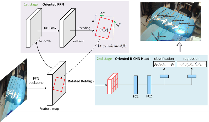
Figure 4: Overall framework of oriented R-CNN [8] consists of two stages. The first stage generates oriented proposals by oriented RPN and the second stage is oriented R-CNN head to classify proposals and refine their spatial locations.

6.  Experiments and Results

This chapter provides a detailed description of the structure of our novel endoscope dataset used for training and testing purposes. A description of the various experiments carried out and the resources used in training our models. We conducted an ablation study using the results from several experiments performed on our dataset to prove the feasibility and measure the performance of the modified and unmodified YOLOv5 models in recognizing surgical instruments from endoscope videos. Finally, we show the results from training and testing our novel endoscope dataset with our benchmark models and compare them with the top four models from our ablation study.

Dataset Structure

Our novel endoscope dataset was extracted from two endoscope videos, which we term Pilot 1 and Pilot 2. From Pilot 1, we annotated seven hundred and seventy-six image frames, and two thousand, six hundred and eighty-nine image frames were annotated from Pilot 2. See Figure 4. Each image frame has a corresponding text file which holds the coordinates of the ground truth annotation for each image. This file is saved in a different folder but in the same directory. In order to split our novel endoscope dataset into training and testing sets, we designed a python script to randomly extract 70% of Pilot 1 and Pilot 2 as the training sets, and the remaining 30% of Pilot 1 and Pilot 2 were used as the test sets. This resulted in our training set consisting of 2425 image frames and their corresponding annotations and our test set consisting of 1040 image frames and their corresponding annotations. Figure 5 displays the distribution of annotation per surgical instrument category from Pilot 1 and Pilot 2.

 

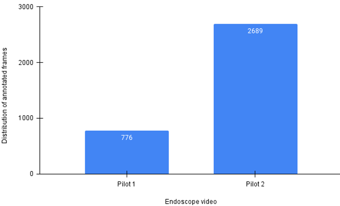
Figure 5: A figure showing the distribution of the number of annotated frames in Pilot 1 and Pilot 2 endoscope videos.

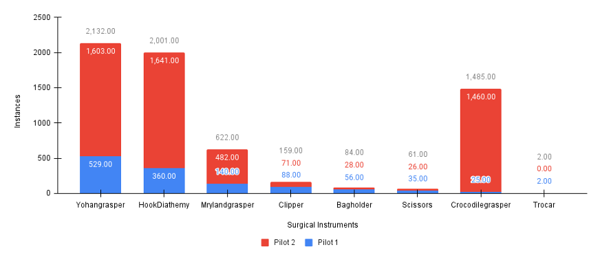
Figure 6: A figure showing the distribution of the samples per surgical instrument category in Pilot 1 and Pilot 2 endoscope videos.

Experimental Setup

The training and testing of all experiments were performed on the Visual Artificial Intelligence Laboratory beta-mars server with an Ubuntu 20.04 operating system and PyTorch framework. The server has four Nvidia GTX 1080 GPUs, each of which has 12 GB VRAM. The training time for each experiment took an average of six hours to complete.

Hyperparameter Settings

In deep learning problems such as this one, hyperparameter setting is a fundamental task that is required in order to improve model performance. The grid search approach for selecting the best hyperparameter value for a model is often utilized during model training. However, a major downside to this approach is that it requires a significant amount of runtime to train across all possible hyperparameter values, thus increasing the computational complexity of the model. Due to time constraints and limited access to computing resources, only a few hyperparameters were manually adjusted to select the best-performing model. Table 1 displays the final values for selected hyperparameters used for training all models.

Table 1: Hyperparameters for experiments

Hyperparameter	Value
Learning rate start	01
Learning rate end	1
Flipud	5
Weight rate decay	0005
Momentum	937
Batch size	16
Epochs	300
Optimizer	Stochastic gradient descent

Ablation Study

In order to illustrate the efficacy of our proposed refinements made to the YOLOv5 algorithm, we conducted an ablation study to demonstrate the effectiveness of each modification in an incremental manner using our novel endoscope dataset and YOLOv5l as our baseline model. F1 score, mAP@0.5, mAP@0.5:0.95, and inference are used as our evaluation metrics. The results of all experiments conducted are summarized in Table 2 below.

Table 2: R An ablation study of model refinements on our novel endoscope dataset. We report the F1-Score, mAP@0.5 IOU, mAP@0.5:0.95 IOU, parameters, and the inference time.  

	Backbone	Neck	Anchors	Size	F1 score	mAP@0.5	mAP@0.5:0.95	Parameters	Inference (ms)
A	CSPDarknet53	PANet	Predefined	640	90	981	6	46145973	4
B	CSPDarknet53	PANet	3	640	94	983	607	46145973	5
C	CSPDarknet53	PANet	5	640	95	978	628	46192643	5
D	CSPDarknet53	BiFPN	3	640	93	975	627	46408117	5
E	CSPDarknet53	BiFPN	5	640	96	977	626	46454787	5
F	CSPDarknet53	FPN	3	640	97	98	589	40703157	8
G	CSPDarknet53	FPN	5	640	97	982	571	40749827	7
H	Our backbone	PANet	3	640	95	98	602	95906421	8
I	Our backbone	PANet	5	640	97	98	612	96019651	9
J	Our backbone	FPN	3	640	97	978	585	33039477	6
K	Our backbone	FPN	5	640	97	976	606	33086147	7

 

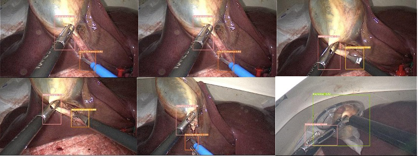
Figure 6: Samples of visualization results of surgical instrument detection using our model. Different colored bounding boxes represent different class categories in our dataset

Model A: To begin with, we build our baseline model using the original design of the YOLOv5 algorithm, which has predefined anchors. This resulted in mAP (98.1%), F1-score (90%), mAP@0.5 (98.1%) and inference speed (9.8ms). 

Model B and C: Model B is the first refinement with a positive effect on the YOLOV5 algorithm, and it involves replacing the predefined anchors with three auto-anchor genetrators. Auto-anchors is a technique introduced in YOLOv5 which helps the algorithm automatically learn the best anchor box for any given dataset. This boosted performance from 98.1% mAP to 98.3% mAP. Model C refinement is similar to model B, except that we used five auto-anchor generators. The model resulted in 97.8% mAP, which is slightly lower than model B and our baseline model. Models B and C are slightly slower than model A.

Model D and E: In these models, the refinements made were replacing the baseline YOLOv5 neck architecture, PANet with BiFPN, and experimenting with three and five auto-anchor generations. Both models resulted in mAP (97.5% and 97.7%) which are lower than our baseline model but achieve a higher F1-score when compared to our baseline model. Both models also achieved higher inference speeds when compared to our baseline model.

Model F and G: The refinements made in these models are similar to those made in models D and E except that we used a different neck architecture, FPN. While model F achieved a slightly lower mAP (98.0%) compared to our baseline model, model G achieved a slightly higher mAP value (98.2%) than our baseline model, which makes it the second refinement with a positive effect on the YOLO algorithm. Both model F and G achieve higher inference speed than our baseline model.

Model H and I: The refinements made in models H and I involved replacing the backbone of our baseline model with our light-weight backbone inspired by VGG and experimenting with three and five auto-anchor generation. Both models achieved the same mAP value 0.98% which is slightly lower than our baseline model, but had a higher inference speed and F1-score when compared to our baseline model.

Model J and K: The refinements made to models J and K are similar to models H and I except that we replace the PANet neck architecture in models H and I with an FPN neck architecture, experimenting with three and five auto-anchor generations. While both models J and K achieved mAP values (97.8% and 97.6%) slightly lower than our baseline model, both models were faster than our baseline model and also achieved an F1-score higher than that of our baseline model.

Comparison with Benchmark Models

In this section, we compare the top four models' performances from our ablation studies in Table 2 with four other state-of-the-art object detection models that can be used for surgical instrument detection tasks. Table 3 displays the comparison results summary while Table 4 displays the performance of all the different experiments conducted in terms of their mean average precision (mAP) at 50% IOU threshold for each surgical instrument in our novel endoscope dataset. The results from Table 3 demonstrate that model B, which is the best performing model from our ablation studies in Table 4, outperformed all our benchmark models except for YOLOv3-SPP, which achieved equal model performance in terms of the mAP value.

Table 3: Table. The comparative results of the speed and accuracy of the top four model performances from our ablation studies with four other state-of-the-art object detection algorithms.

Model	F1 score	mAP@0.5	mAP@0.5:0.95	Parameters	Inference
YOLOv7	97	98	617	36519530	7
YOLOv3-SPP	93	983	513	62584213	3
Scaled-YOLOv4	81	836	469	52501333	8
YOLOR	86	832	47	36844024	5
B	94	983	607	46145973	5
G	97	982	571	40749827	7
A	90	981	6	46145973	4
I	97	98	612	96019651	9

Table 4: Results comparing mAP@0.5 value for each surgical instrument for the different model experiments conducted.

Model	Crocodile grasper	Johan grasper	Hook diathermy	Maryland grasper	Clipper	Scissors	Bag holder	Trocar
A	978	956	978	986	995	995	961	995
B	977	965	981	995	955	995	962	995
C	971	943	979	984	995	995	958	995
D	968	947	978	978	995	995	946	995
E	975	94	978	984	995	955	955	955
F	97	952	982	984	995	995	965	995
G	977	96	986	986	995	995	962	995
H	974	949	976	99	995	995	965	995
I	961	956	981	991	995	995	964	995
J	951	95	986	995	995	995	959	995
K	95	953	979	984	995	995	96	995
YOLOv7	981	961	985	983	996	972	966	955
YOLOv3-SPP	983	96	977	995	995	995	964	995
Scaled-YOLOv4	939	928	974	975	995	976	901	0
YOLOR	969	948	976	981	995	968	818	0

Rotated Surgical Tools Detection Results

This section provides both the quantitate and qualitative results of our rotated object detection model. Table 5 shows the performance of each class in terms of recall and average precision including the mAP for all classes. In addition, we also visualised the performance of our rotated tools detector model in Figure 7, where we showed both the tips of the tools and entire tool.

Table 5: Results of our rotated object detection model for all classes with IoU threshold of 0.5.

Classes	Gts	Dets	Recall	Average precision
Clipper	7	35	286	182
Crocodile grasper	11	21	727	655
Hook diathermy	6	36	00	939
Maryland grasper	21	91	05	886
Scissors	18	58	944	868
Surgical instrument	1787	2478	628	471
Trocar	162	469	623	506
Johan grasper	31	81	935	894
mAP				675

 Figure 7: Visual results of surgical instruments and their tips detection using our rotated objection detection model.

References

[1]	Bochkovskiy, Alexey, Chien-Yao Wang, and Hong-Yuan Mark Liao. "Yolov4: Optimal speed and accuracy of object detection." arXiv preprint arXiv:2004.10934 (2020).
[2]	Thuan, Do. "Evolution of Yolo algorithm and Yolov5: The State-of-the-Art object detention algorithm." (2021).
[3]	Katsamenis, Iason, Eleni Eirini Karolou, Agapi Davradou, Eftychios Protopapadakis, Anastasios Doulamis, Nikolaos Doulamis, and Dimitris Kalogeras. "TraCon: A novel dataset for real-time traffic cones detection using deep learning." In Novel & Intelligent Digital Systems Conferences, pp. 382-391. Springer, Cham, 2023.
[4]	Simonyan, Karen, and Andrew Zisserman. "Very deep convolutional networks for large-scale image recognition." arXiv preprint arXiv:1409.1556 (2014).
[5]	Krizhevsky, Alex, Ilya Sutskever, and Geoffrey E. Hinton. "Imagenet classification with deep convolutional neural networks." Communications of the ACM, 60, no. 6 (2017): 84-90.
[6]	Lin, Tsung-Yi, Piotr Dollár, Ross Girshick, Kaiming He, Bharath Hariharan, and Serge Belongie. "Feature pyramid networks for object detection." In Proceedings of the IEEE conference on computer vision and pattern recognition, pp. 2117-2125. 2017.
[7]	Tan, Mingxing, Ruoming Pang, and Quoc V. Le. "Efficientdet: Scalable and efficient object detection." In Proceedings of the IEEE/CVF conference on computer vision and pattern recognition, pp. 10781-10790. 2020.
[8]	Xie, Xingxing, Gong Cheng, Jiabao Wang, Xiwen Yao, and Junwei Han. "Oriented R-CNN for object detection." In Proceedings of the IEEE/CVF International Conference on Computer Vision, pp. 3520-3529. 2021.